What are you looking for?
What Is Modulation Transfer Function?
Definition of Modulation Transfer Function
The Modulation Transfer Function (MTF) is a performance metric that measures the degradation of contrast in the image compared to contrast in the object. As contrast degrades, observers find it increasingly hard to distinguish small features in the image. There are several factors that cause contrast degradation, such as diffraction effects, optical aberrations, and vignetting. Therefore, you can use the MTF to evaluate and compare optical systems.
Table of Contents
Determining the System MTF
To determine the system MTF, you can use a sinusoidal pattern with perfect contrast as the object. Image contract is designed as:


where Imax and Imin are maximum and minimum irradiances, respectively. The maximum value the contrast can take is 1, and the minimum value is 0.
A cycle of the sinusoidal pattern corresponds to a black and a white fringe. Each cycle is also referred to as a line pair (lp). Spatial frequency is often measured in line pairs or cycles per unit distance, which is typically mm. Thus, the spatial frequency unit is commonly represented as lp/mm or cycles/mm. For afocal systems, the units are converted to angular frequencies, typically measured in cycles/milliradian.


Figure 1. An optical system causes contrast degradation in the image with respect to contrast in the object.
Figure 1 shows the response of the system to a single frequency, however, the MTF measures the response for continuous frequencies up to the cutoff frequency fc. The cutoff frequency, which is the highest frequency the system can resolve, is given by:


The MTF is a function of a 2D spatial-frequency vector, but it is usually presented as a 1D plot. In this type of representation, it is useful to compare the response to that of a perfect system. In an aberration-free system, the contrast is only degraded by diffraction effects. The dotted line in Figure 2 shows the MTF for the aberration-free system, which is labeled as “Diffraction Limit.”


Figure 2. On-axis MTF plot of an optical system compared to the diffraction-limited MTF plot. The output image depicts excellent contrast at low frequencies and poor contrast at high frequencies, mimicking the MTF plot.
For off-axis field points, the MTF result depends on the orientation of the bar pattern. It is common to show the tangential (T) and radial directions (R) for each field point, as shown in Figure 3. In a tangential target, the bars are tangent to the image circle, and in a radial target, the bars are parallel to the radial direction.


Figure 3. Off-axis MTF plots for the tangential and radial directions. In CODE V, the target bars are relative to the Y axis. Radial MTF corresponds to vertical bars and tangential MTF corresponds to horizontal bars.
It is sometimes useful to measure through-focus MTF, which shows the MTF for selected frequencies as a function of defocus position. Another informative MTF chart is MTF vs. field points, which shows the MTF for selected frequencies as a function of field points. Examples of these plots are shown in Figure 4.
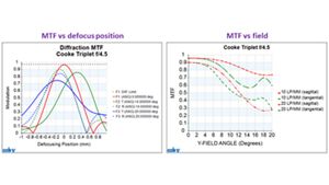

Figure 4. Examples of MTF vs. defocus position (left) and MTF vs. field (right) charts.
Contrast Transfer Function
So far, we have described sine-wave targets that represent a single frequency. The response of the system to a square-wave pattern is called Contrast Transfer Function (CTF). The CTF may be a more appropriate performance metric for systems that image objects with square-wave features, such as barcode readers. Computationally, you can approximate the CTF by summing a series of sine wave response values.
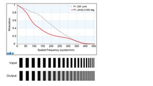

Figure 5. On-axis CTF. The target is a square-wave pattern instead of a sine-wave pattern.
MTF Considerations During the Design Process
The optical designer doesn’t necessarily aim to achieve the diffraction limit performance. The desired MTF curve is based on design requirements. The lens specifications usually take the form of an MTF value for specific frequencies. The MTF specification may come, for instance, from the sensor pixel size and the Nyquist theorem, which describes the maximum spatial frequency that the sensor can resolve.
For example, assume a digital sensor with a pixel size of 7.4 μm x 7.4 μm. According to the Nyquist theorem, the highest frequency that can be resolved is 1 cycle/(2 x 7.4 um) = 0.0676 cycles/μm ≈ 68 cycles/mm. Based on the sensor characteristics, a typical performance requirement for the lens could be:
- MTF > 50% at 17 cycles/mm, and
- MTF > 25% at 68 cycles/mm.
Figure 6 shows the MTF chart from a lens that would meet these requirements for all fields. It is important to know the sensor characteristics during the design process because in many cases the Nyquist frequency of the sensor is only a small fraction of the diffraction cutoff frequency fc.


Figure 6. System that meets requirements of MTF > 50% at 17 cycles/mm and MTF > 25% at 68 cycles/mm.
Another useful consideration is that for small aberrations, the degradation of the MTF occurs near half the diffraction cutoff frequency. This is because the MTF at zero frequency is always unity and the MTF at the diffraction cutoff frequency is zero. If you measure the aberrated MTF as a ratio of the aberration-free MTF, the result is a function that sags down in the middle.
How Do You Measure the MTF in Practice?
Experimentally, you can measure the frequency response of an optical system in different ways, for example, using the slanted-edge target or the three-bar target. These targets are easy to use because they just need to be imaged.
The three-bar target is a common method to measure resolution. It consists of three parallel bars of certain width and separation that corresponds to a specific spatial frequency. To measure system resolution, arrange multiple three-bar patterns at specific frequencies in a single chart and inspect the resulting image to determine the smallest features you can resolve.
A popular target with these characteristics is the USAF 1951 chart shown in Figure 7. The measured resolution from a three-bar target might differ from the predicted CTF, because the CTF assumes an infinitely long pattern of bars. In a pattern with a finite number of bars, you may see end effects that reduce the contrast of the bars at the ends of the pattern. For this reason, the measured contrast might be less than predicted by the CTF.
Another method to experimentally measure the MTF is the slanted-edge target. This method is different in that you can obtain frequency information from a single target. In this method, you must set the edge at a specified small angle with respect to the pixel array of the sensor, as shown in Figure 7. When the input is a step function instead of a point source, the irradiance distribution at the image is an edge spread function. You can then determine the MTF from the Fourier transform of the derivative of the edge spread function.


Figure 7. Examples of targets that can measure MTF experimentally, with a three-bar chart (left) and slanted-edge target (right).
How Do You Compute the MTF?
To determine how to compute MTF, first you need to define the Point Spread Function (PSF), the Transfer Function (TF), and their relationship with the MTF.
The Point Spread Function (PSF) of an imaging system is the resulting irradiance distribution when the object is a point source. For coherent light, the PSF is related to the Fourier transform of the pupil function’s complex amplitude. For incoherent light, the PSF is related to the Fourier transform of the pupil function’s intensity. Therefore, the coherent and incoherent PSF relate as follows.
Where r is a 2D spatial-position vector:


The incoherent transfer function r of a linear, shift-invariant system is given by the Fourier transform of the incoherent point spread function:


where p is a 2D spatial-frequency vector and F2 denotes a 2D Fourier transform. The transfer function can then be written in terms of the coherent PSF as:


The coherent pupil function pf(r) is the complex amplitude of the wavefront at the exit pupil sphere. Its phase (relative to the reference sphere) is given by the aberrations, and the amplitude is either unity inside the pupil boundary or determined by a specific apodizing function.
Because the coherent PSF is related to the Fourier transform of the coherent pupil function pf(r), the transfer function can also be written as:


where B is a constant factor that depends on the source wavelength and the distance between the point source and the pupil, and the star ⋆ denotes autocorrelation. Thus, the incoherent transfer function is related to the complex autocorrelation of the pupil function. It is convenient to normalize the transfer function relative to TF(0). The result is referred to as the Optical Transfer Function (OTF):


The Modulation Transfer Function (MTF) is the modulus of the optical transfer function:


Therefore, you can compute the MTF by calculating the complex autocorrelation of the pupil function, or by computing the Fourier transform of the incoherent PSF. Using the definition of the MTF, the OTF can be written in complex form as:


where p(p) is the phase. The MTF can only take positive values, but the OTF can be negative when there is phase reversal. For the image of the bar pattern, this would result in contrast reversal, meaning that white features become dark and dark features become light.
In an MTF plot, the MTF curve reaches zero and then “bounces.” It is important to be aware of this behavior. After the bounce, the MTF technically increases even though it reached zero at a lower frequency. Another possible impact is that if the MTF is used in the error function during optimization, phase reversal may produce local minima.
Other common system specifications are Strehl ratio and RMS wavefront error. For small aberrations, specifying the Strehl ratio is equivalent to specifying the RMS wavefront error. The Strehl ratio is defined as the ratio of the peak intensity of the measured PSF to the peak intensity of the perfect PSF. The MTF is related to the inverse Fourier transform of the incoherent PSF.
As a result, you can express the Strehl ratio as the integral under the entire MTF curve, including frequencies beyond the Nyquist frequency (which are irrelevant). For this reason, in situations where Nyquist is well below the diffraction cutoff, it makes more sense to specify MTF at frequencies between zero and the Nyquist frequency, rather than specifying the Strehl ratio or RMS wavefront error.
Using CODE V
CODE V is a powerful optical design tool. Its advanced analysis tools include the computation of the MTF by evaluating the autocorrelation of the pupil function and the computation of the CTF by calculating a series summation of sine wave response values.
Level Up Your Optical Designs with CODE V
CODE V uses MTF metrics throughout the design process for analyzing, optimizing, and tolerancing optical systems.


References
Explore related blogs


Want help or have questions?