Resource Guide
Engineers Guide to Digital Signal Processing


Introduction
You run a radar or high-speed link test that should look clean. The waveform on the scope seems fine, but the frequency plot tells a different story. Spurs appear. The noise floor rises. A peak shows up where it shouldn’t. At that point, most engineers ask the same question. Is the signal actually bad, or did the measurement setup miss something?
This situation is common in RF, automotive radar, 5G, and high-speed digital work. Problems in the measurement chain can alter the signal before analysis begins, making later results misleading. Digital signal processing helps separate real signal behavior from measurement artifacts and cuts down time spent chasing false issues.
This guide covers DSP fundamentals and practical measurement workflows. From capturing clean signals to analyzing them in the frequency domain and validating results. You’ll see how sampling choices, triggering, and basic DSP techniques work together in real test scenarios, with a focus on reducing measurement errors and improving confidence in your results.
Background and Context
Digital signal processing sits at the intersection of mathematics, measurement hardware, and real-world signals. It gives you a structured way to analyze signals that change over time, especially when those signals become too fast, noisy, or complex to evaluate by inspection alone.
Several core concepts appear repeatedly in DSP workflows:
- Sampling rate defines how often a signal is captured in time. Under the Nyquist sampling theorem, the sampling rate must be at least twice the highest frequency component to prevent aliasing. In practice, engineers often use 2.5–5× margin.
- Fast Fourier Transform (FFT) converts time-domain data into the frequency domain, exposing harmonics, spurs, and noise that are difficult to see otherwise.
- Z-transform extends frequency analysis to discrete-time systems and underpins digital filtering and stability analysis.
DSP plays an important role across multiple industries. In telecom applications, it supports modulation analysis and interference detection. In aerospace and defense, it enables radar processing, pulse analysis, and phase measurements. In semiconductor and high-speed digital design, DSP helps evaluate signal integrity, jitter, and bit error behavior as data rates increase.
DSP is also commonly misunderstood. Engineers often skip windowing during FFT analysis, which causes spectral leakage and misleading frequency results. Others treat DSP as a software-only task and overlook how probes, grounding, triggering, and sampling affect the data before any math occurs.
To use DSP effectively, you need a working understanding of Fourier concepts and comfort with oscilloscope operation. If you want a quick refresher on the measurement fundamentals that feed DSP analysis, the oscilloscope basics guide provides helpful context on bandwidth, sampling, and triggering.
Step-by-Step Instructions
DSP works best when you follow a consistent workflow. Each step builds on the one before it, starting with signal capture and ending with validation. Skipping steps or changing their order often leads to misleading results, especially in RF, radar, and high-speed digital applications.
The workflow below reflects how engineers typically move from raw measurements to reliable DSP analysis using modern oscilloscopes and analyzers.
Overview: 7-step DSP workflow
| Step | Description | Difficulty | Typical time |
|---|---|---|---|
| 1 | Signal capture | Easy | ~5 min |
| 2 | FFT setup | Medium | ~10 min |
| 3 | Windowing | Medium | ~8 min |
| 4 | Filtering | Hard | ~15 min |
| 5 | Convolution | Hard | ~20 min |
| 6 | BER analysis | Hard | ~25 min |
| 7 | Validation | Medium | ~12 min |
Step 1: Capture quality signals
DSP accuracy starts with the capture. Trigger stability, probe selection, and sampling rate all determine whether the data entering the DSP chain represents the real signal or a distorted version of it.
For time-domain capture, configure triggering to lock onto the event of interest and confirm that the sampling rate comfortably exceeds the highest frequency component of the signal.
Pay close attention to probes and connections. Probe bandwidth, attenuation, and loading directly affect amplitude and rise time. Poor grounding or long ground leads can introduce noise that later appears as false frequency components.
Tips and warnings
- Sample above the Nyquist limit with margin to reduce aliasing
- Match probe bandwidth to the signal under test
- Minimize ground loop area to limit noise pickup
Probe right and trigger deliberately. Clean capture prevents aliasing from appearing later as a DSP problem.
Step 2: Apply FFT transform
Once the signal is captured correctly, you can move from the time domain to the frequency domain using an FFT. This step reveals harmonics, spurious tones, and broadband noise that are difficult to see in the waveform view alone. FFT settings such as span, resolution bandwidth, and scaling affect how clearly these components appear.
Trigger stability remains important here. Any timing jitter in the capture can smear frequency components and raise the apparent noise floor. For a refresher on stable triggering methods, see the oscilloscope triggering guide. For deeper theory behind FFT behavior and interpretation, the FFT application note provides useful background.
Step 3: Apply windowing to reduce spectral leakage
After running an FFT, windowing becomes critical for interpreting frequency-domain results accurately. When a captured signal does not contain an integer number of cycles within the time record, sharp edges form at the record boundaries. These edges spread energy across the spectrum, a problem known as spectral leakage.
Windowing smooths those edges before the FFT runs. Common windows such as Hanning, Hamming, or Flat Top balance frequency resolution against amplitude accuracy. No single window works best for every case, so the choice depends on whether you care more about precise frequency location or accurate amplitude measurement.
Key considerations
- Use narrower windows for better frequency resolution
- Use Flat Top windows when amplitude accuracy matters
- Keep window choice consistent when comparing measurements
Common mistake
Applying FFTs without windowing and assuming spurs or noise are part of the signal.
Windowing does not fix a bad capture. It prevents clean signals from looking worse than they are.
Step 4: Apply digital filtering
Filtering helps isolate the part of the signal you actually want to analyze. In DSP workflows, digital filters often remove out-of-band noise, suppress interference, or extract specific frequency components before further processing.
You can apply low-pass, high-pass, band-pass, or notch filters depending on the signal and application. Aggressive filtering can distort phase or smear transient behavior, especially in time-sensitive measurements like pulse analysis or eye diagrams.
Best practices
- Set cutoff frequencies with margin around the signal of interest
- Use lower-order filters when phase accuracy is important
- Verify filtered results against the unfiltered signal
Filtering works best when used conservatively. The goal is to clarify the signal, not reshape it.
Step 5: Perform convolution for signal and system analysis
Convolution allows you to understand how a system responds to a given input. In practical terms, it combines a signal with an impulse or response function to predict output behavior. Engineers use convolution to model channel effects, analyze impulse responses, or correlate known patterns within noisy data.
In multi-channel environments, convolution helps compare timing, phase, and correlation between signals. This becomes especially useful in radar processing, sensor fusion, and synchronized digital systems.
Typical use cases
- Channel response analysis
- Pulse compression in radar
- Time-aligned signal comparison
Because convolution amplifies both signal and noise, it works best after careful capture and filtering.
Step 6: Analyze bit error rate (BER)
For high-speed digital links, BER analysis provides a quantitative measure of signal quality. BER reflects how often bits are received incorrectly over a given time or data volume. Even small impairments such as jitter, crosstalk, or attenuation can dramatically increase error rates.
DSP techniques support BER analysis by conditioning the signal, aligning clocks, and separating deterministic effects from random noise. Eye diagrams, jitter decomposition, and pattern analysis often feed directly into BER measurements.
What to watch
- Long enough test duration to capture rare errors
- Stable triggering and clock recovery
- Correlation between BER spikes and spectral artifacts
BER analysis often exposes problems that do not appear in simple time- or frequency-domain views.
Step 7: Validate results against known behavior
Validation confirms that the DSP workflow clarified the signal instead of introducing new artifacts.
This step may include repeating measurements with different settings, cross-checking results in the time and frequency domains, or comparing data across channels or instruments.
Validation checks
- Results remain consistent across captures
- DSP output matches theoretical expectations
- Changes in setup produce predictable changes in results
If a result cannot be reproduced or explained, it is not ready to guide design decisions.
Troubleshooting
When DSP results do not match expectations, the cause usually appears earlier in the measurement chain. Most issues stem from setup problems rather than the DSP math itself. The following errors account for the majority of misleading results seen in real test environments.
Common user errors
- Probe capacitance and loading that distort fast edges and reduce amplitude accuracy, sometimes by 20 percent or more
- Probe mismatch from incorrect attenuation settings or insufficient bandwidth
- Aliasing from undersampling, where higher-frequency content folds into lower frequencies
- FFT leakage caused by missing or inconsistent windowing
- Noise spikes from EMI, often introduced through poor grounding or cable routing
Each of these issues can alter the signal before analysis begins. Once that happens, FFTs, filters, and BER calculations amplify the error rather than reveal the true signal behavior.
How to correct most DSP issues
- Confirm probe type, attenuation, and bandwidth before capturing data
- Increase sampling rate and verify Nyquist margin
- Apply windowing consistently when using FFTs
- Minimize ground loop area and improve shielding
- Compare time- and frequency-domain views to validate results
When to seek help
If results remain inconsistent after correcting setup and DSP parameters, hardware accuracy may be the limiting factor. Component aging, drift, or undocumented adjustments can undermine measurement confidence. In these cases, verified calibration becomes essential.
Advanced Tips and Variations
Once you are comfortable with the core DSP workflow, small changes in technique or tool selection can unlock deeper insight and reduce debug time. Advanced DSP becomes most valuable when signals operate close to their limits, such as high-speed serial links, radar systems, and multi-channel automotive networks.
High-Speed Links and BER Analysis
DSP precision is critical in bit error rate testing for interfaces like PCIe. Error rates can fall well below what short tests reveal, often reaching 10⁻¹² BER or lower. Measuring at this level requires long capture times, stable clock recovery, and consistent DSP conditioning. Small differences in filtering, jitter handling, or alignment can determine whether a link passes or fails.
Key factors to watch:
- Sufficient test duration to capture rare errors
- Stable triggering and clock recovery
- Correlation between BER events and spectral behavior
Multi-Channel and MIMO Analysis
Multi-channel systems introduce timing and phase challenges that single-channel analysis cannot expose. MIMO radar and sensor systems depend on tight synchronization across channels. DSP applied across synchronized inputs helps identify channel skew, phase drift, and correlation errors that would otherwise go unnoticed. This approach is common in radar, ADAS, and sensor fusion workflows.
DSP Beyond RF: Automotive Networks
DSP techniques also apply outside traditional RF analysis. CAN and other automotive networks benefit from filtering and frequency-domain analysis to isolate noise, intermittent faults, and timing violations. Combining protocol decoding with DSP often reveals interference sources that raw waveforms alone fail to show.
MATLAB vs Hardware-Based DSP
Many engineers prototype DSP algorithms in MATLAB or similar tools. Software excels at modeling and simulation, while hardware-based DSP captures real-world effects such as jitter, coupling, and noise. In practice, combining both approaches delivers the most reliable results: hardware for accurate capture, software for deeper exploration.
Customizing DSP Workflows Under Deadlines
When schedules are tight, DSP customization helps keep projects on track. Narrowing analysis to critical frequency bands, shortening capture windows, or simplifying filter stages can reduce processing time without sacrificing confidence.
For engineers who want to strengthen their theoretical foundation alongside practical work, the IEEE Signal Processing Society lecture notes offer applied DSP tutorials and real-world examples. You can explore them through the IEEE DSP tutorial library, which pairs well with measurement-driven DSP workflows.
Real-World Applications
DSP shows its value most clearly when it is applied to real measurement problems rather than abstract signals. Across industries, engineers use DSP to clarify behavior, isolate faults, and validate performance in situations where time-domain views alone fall short.
Common applications where DSP is used effectively
- ADAS radar: Engineers rely on DSP to analyze chirps, Doppler shifts, and phase behavior in automotive radar systems. Frequency-domain analysis helps separate real targets from noise and interference, while multi-channel DSP supports alignment and correlation checks in sensor fusion workflows.
- 5G and high-speed wireless testing: DSP enables modulation analysis, spectral evaluation, and error detection in complex waveforms. Techniques such as FFT analysis and filtering help engineers identify interference, distortion, and timing issues that affect link quality and throughput.
- Powertrain and inverter debugging: In electric and hybrid vehicles, DSP helps isolate switching noise, harmonics, and transient events in motor drives and power electronics. Frequency analysis often reveals coupling and EMI sources that remain hidden in time-domain captures.
- EMC and EMI investigation: DSP supports pre-compliance testing by identifying dominant emission frequencies and tracking noise sources back to their origin.
While DSP provides deeper insight, it also has practical limits. Real-time constraints, finite memory depth, and processing latency can restrict how much data you can analyze at once. Engineers often balance capture length, resolution, and processing complexity to stay within these limits while still extracting meaningful results.
For automotive-focused measurements, including radar, power electronics, and in-vehicle networks, the automotive oscilloscope guide outlines instrument considerations that directly affect DSP workflows, such as bandwidth, channel count, and synchronization.
Additional Resources
If you want to deepen your DSP knowledge beyond day-to-day measurements, a mix of theory, community discussion, and practical guides works best.
Further learning
- Understanding Digital Signal Processing by Richard G. Lyons is a widely used reference for engineers who want clear explanations without unnecessary abstraction.
Read more about the book here: Understanding Digital Signal Processing by Richard G. Lyons - Structured academic refreshers are available through Coursera’s university-led programs, including EPFL’s DSP courses: Digital Signal Processing courses on Coursera
Community and discussion
- The IEEE Signal Processing Society publishes applied tutorials and lecture notes that connect DSP theory to real engineering problems: IEEE Signal Processing Society lecture notes
- Engineers regularly share FFT plots, windowing questions, and debugging advice in the DSP community on Reddit: r/DSP community discussions
Measurement-focused guides
- A practical refresher on signal capture fundamentals that support DSP workflows: Oscilloscope basics guide
- Guidance on calibration, traceability, and maintaining measurement confidence: Calibration certificates guide
These resources help connect DSP theory with the measurement challenges you encounter at the bench.
Conclusion
This guide walked through a practical seven-step DSP workflow, from capturing clean signals to validating results you can trust.
When you apply DSP correctly, you gain three clear benefits:
- better visibility into signal behavior
- faster root-cause analysis
- more confident design and test decisions.
Instead of guessing whether an issue comes from the signal or the setup, DSP helps you separate the two and move forward with clarity.
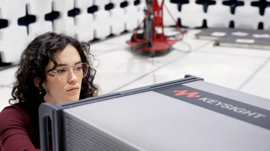
If you want reliable performance without paying new-equipment prices, the Keysight Used Equipment Store offers Premium Used oscilloscopes, spectrum and network analyzers, BERTs, RF power meters, and sensors. Each instrument is OEM-calibrated, backed by a warranty, and supported by experts who understand real testing challenges.
When accuracy, turnaround time, and budget all matter, choosing the right equipment now helps keep your work moving forward without unnecessary delays.
Whenever You’re Ready, Here Are 5 Ways We Can Support Your Capacitor Projects
Call tech support US: +1 800 829-4444
Press #, then 2. Hours: 7am – 5pm MT, Mon– Fri
Contact our sales support team
Create an account to get price alerts and access to exclusive waitlists
Talk to your account manager about your specific needs.
FAQs
Can used Keysight equipment handle real-time DSP analysis?
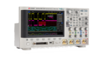
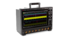
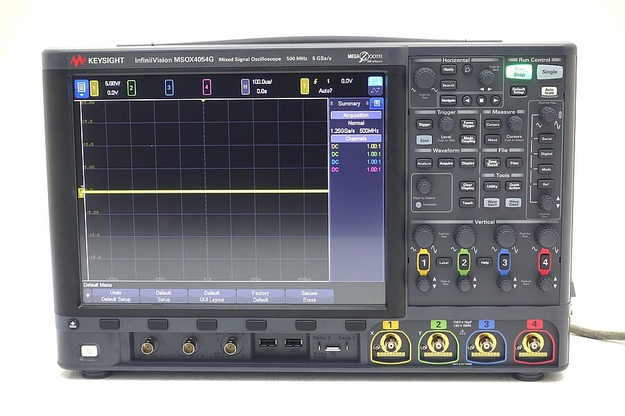
Yes. Used Keysight MSOX and MXR Series oscilloscopes support real-time capture with built-in FFT, filtering, and analysis features suitable for 5G, radar, and high-speed digital work. Because certified used units include OEM calibration, sampling rate and timing accuracy remain reliable for DSP tasks.
What’s the minimum bandwidth needed for 5G DSP testing?
For sub-6 GHz 5G applications, engineers typically start with 1 GHz or more of bandwidth to maintain sampling margin. For mmWave analysis, significantly higher bandwidth is required.
How do I choose between MSOX and MXR series for DSP?
The MSOX series offers a cost-effective 4-channel option for general DSP tasks such as FFT analysis, filtering, and protocol debugging. The MXR series adds higher bandwidth and up to 8 channels, which is valuable for MIMO radar, multi-channel correlation, and advanced automotive DSP workflows.
What’s the warranty on refurbished Keysight DSP gear?
Certified refurbished equipment typically includes a one-year warranty, with extended coverage options available. Each unit ships with calibration documentation, which supports measurement confidence comparable to new instruments.
What oscilloscope do I need for DSP?
Most DSP applications benefit from an oscilloscope with at least 1 GHz bandwidth, deep memory, and built-in FFT and digital filtering.
How does FFT work in signal analysis?
An FFT converts time-domain data into the frequency domain, revealing harmonics, spurs, and noise components. This transformation helps engineers understand spectral behavior that is not visible in waveform views alone and supports tasks such as interference analysis and filtering.
What is the Nyquist sampling theorem?
The Nyquist theorem states that a signal must be sampled at least twice its highest frequency component to prevent aliasing. In real measurements, engineers often use a 2.5–5× margin to account for non-ideal signals and filter roll-off.
MATLAB vs hardware DSP tools—which is better?
MATLAB works well for modeling and algorithm development, while hardware-based DSP captures real-world effects like noise, jitter, and coupling. Many engineers use both by exporting measured data into software tools for deeper analysis and validation.
What causes aliasing in signal processing?
Aliasing occurs when a signal is sampled below the required rate, causing higher-frequency components to appear at lower frequencies. This folding effect creates false spectral content that can only be avoided by increasing sampling rate or applying proper filtering.
How do I measure BER with oscilloscopes?
Oscilloscopes support BER-related analysis through eye diagrams and jitter measurements, while dedicated BERT instruments provide precise bit error rate testing for high-speed serial standards. These tools work together to validate link performance down to very low error rates.